2 - Text Classification

ucla | CS 162 | 2024-01-11 23:26

---

Table of Contents

• Classifiers
  • Rule Based Classifier
  • Supervised Classifier
• Probabilistic Classifier
  • Creating the model
  • Bag of Words (BoW) Assumption
  • Naive Bayes Assumption
  • Final Model - MAP prediction
  • Complexity
• Naive Bayes Classifier
  • Learner for NB classifier
  • Prediction
• Practicalities
  • Log Probs
  • Generative vs Discriminative Models
  • Feature Engineering
  • Log Reg Gradients
  • Differences

Classifiers

Rule Based Classifier

• doesn’t generalize, but good for specific corpuses

  Supervised Classifier

• takes inputs $\overrightarrow{x}$ from the corpus and labels $y$ per input as a class and learns from supervised training
• vecotrized: $X=[{\overrightarrow{x}}_1,\dots ,{\overrightarrow{x}}_n]$, $Y=[y_1,\dots ,y_n]$
• a classifier $C:{\overrightarrow{x}}_i\to y_i$
• a learner $L:X\times Y\to C$

  Probabilistic Classifier

• logits = log probs of $p(y

  \vec x)$

• we want our classifier to output $\text{argmax}_y\space p(y

  \vec x)$

• i.e. return the label with the highest probability of being correct and create a model that does this for the most inputs correctly

  Creating the model

• the distribution is a multinomial distribution because of the many classes
• we want to find a direct MLE (maximum likelihood estimation) https://blog.jakuba.net/maximum-likelihood-for-multinomial-distribution/
• i.e. the MLE is the word’s frequency in the corpus so its a terrible estimator because the prediction space is exponentially large
• so we make model assumptions

  Bag of Words (BoW) Assumption

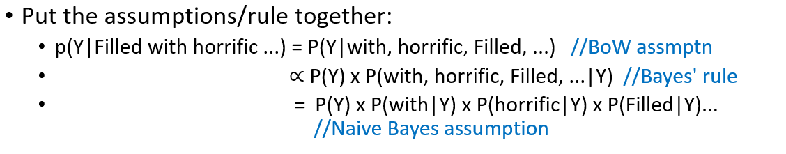
• assume the order of words does not matter i.e. $$p(y

  \text{“Filled with horrific”})=p(y

  \text{“with”,”horrific”,”filled”})$$

• this sets the inputs as a set instead of a sequence
• however this simplifies the problem but introduces new issues in positional context
• but this is still not enough because this represents the sentences as a set but the likelihood this occurs in the corpus is still incredibly low

  Naive Bayes Assumption

• words are independent conditioned on their class

• i.e. the bayes independence formula $$p(\text{“Filled”,”with”,”horrific”}

  y)=p(y)\prod_{x_i\in \vec x} p(x_i

  y)$$

• now we reduce the space to the vocab size (from the corpus to unique words) (from $O(V^n)$)

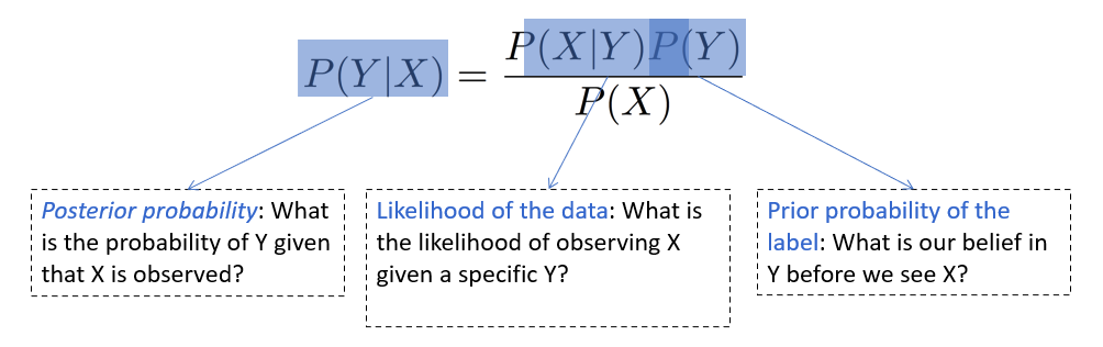
• now to find $p(y

  \text{filled,horrific,with})$ can be solved with bayes rule due to the above assumption to allow us to find each words probs

  • 
• both assumptions brings us to
  • 

    Final Model - MAP prediction

• simplification brings us to:
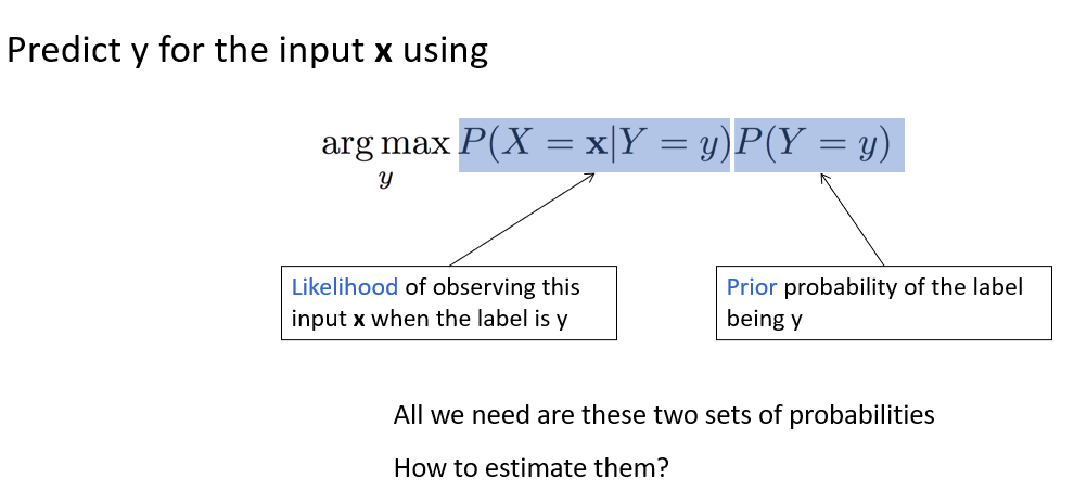
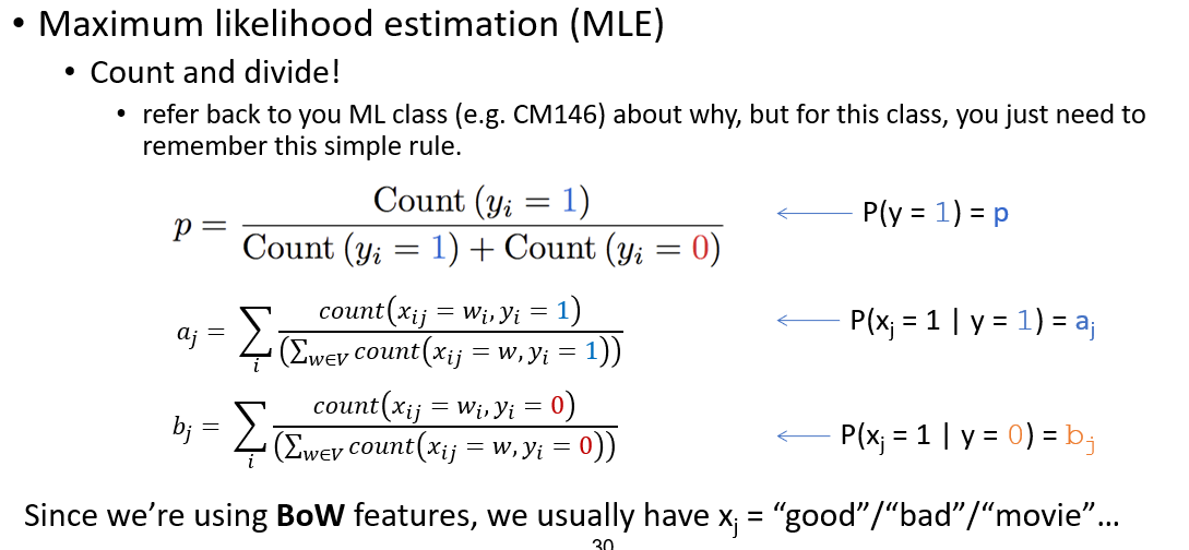
• the prior is the frequency of the label from the multinomial distribution
• the likelihood can be found by counting the occurrences of X=x when Y=y and divide by the overall number of times Y=y

  Complexity

• initially $k-1$ parameters for $k$ classes and $V^n-1$ parameters for $V$ vocab size, the last class and word can be found from not being in the parameters
• now we have only $k(V-1)$ overall parameters

  Naive Bayes Classifier

• using all of these assumptions we can make the following classifier
• assume features (words in sentences) are conditionally independent given the label $y$

• to predict we need the prior $p(y)$ and the likelihood for each $x_j$ for $p(x_j

  y)$,thenwehavetheprediction(hypothesis):$$h_{NB}(\vec x)=\text{arg}\max_y\space P(y)\prod_j P(x_j

  y)$$

• where the term in the prod is (note here we add smoothing for 0 counts)

  Learner for NB classifier

  

  Prediction

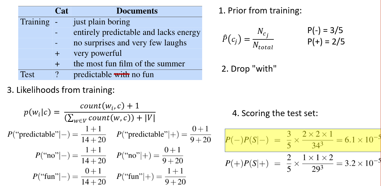
• for prediction we can drop tokens/words that are not in our test input

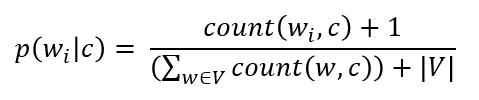
• we can also supply smoothing (regularization) by +1 to numerator of likelihoods and +$

  V

  $ to denominator

• for the denominator likelihood counts, we count the number of words that occur for each label ocurrence
• 

Practicalities

Log Probs

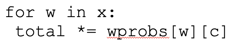
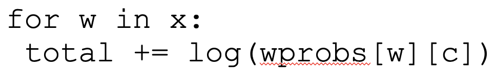
• large vocab size multiplying bayes probs will cause underflow
• instead use logits to represent multiplication of words by probs into sum of log probs
  • 
  • 

    Generative vs Discriminative Models

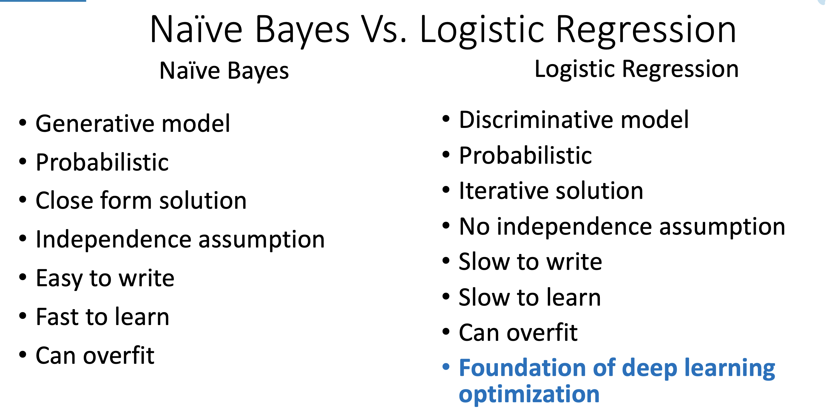
• Generative models learn a joint probability distribution $p(\overrightarrow{x},y)$

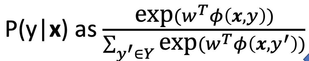
• Discriminative models learn a conditional probability distribution $p(y

  \vec x)$

• naive bayes learns $p(\vec x

  y)\propto p(\vec x,y)$ so its really generative

• so to make $p(y

  \vec x)$fromourcurrentnaivebayesmodel,wecanassumeascoringfunctionforatextinstanceanditslabel$\text w^T\Phi(\vec x,y)$

  • here the weights are ${\text{w}}^T$
  • the feature function $\mathrm{\Phi }(\overrightarrow{x},y)$ is a score not a probability and returns a vector
  • multiplying the 2 gets a scalar
  • we can then take the exponent of the function to make the range $(0,\mathrm{\infty })$ and monotone (nondecreasing)
  • then we can model it is as softmax (or multiclass logistic regressor)
• 
• now we can treat this as a prob maximization by picking best weights

  Feature Engineering

• now given the feature function we need to do some feature selection for $\mathrm{\Phi }$
• n-grams for sequence information
• punctuation, text length, etc.
• then we use a MLE to find max weights
• 
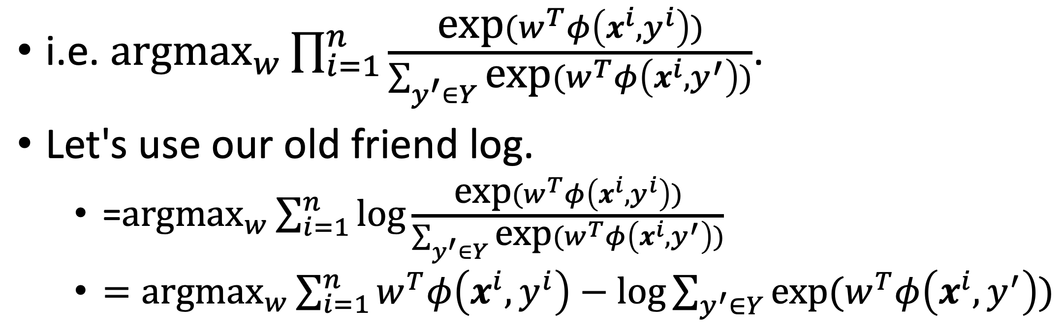
• this is ongruent to mnimizing the negative log likelihood of
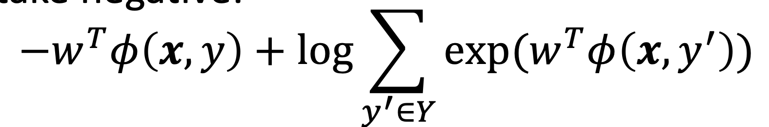
• now wee use gradient descent

  Log Reg Gradients

• the gradient is:
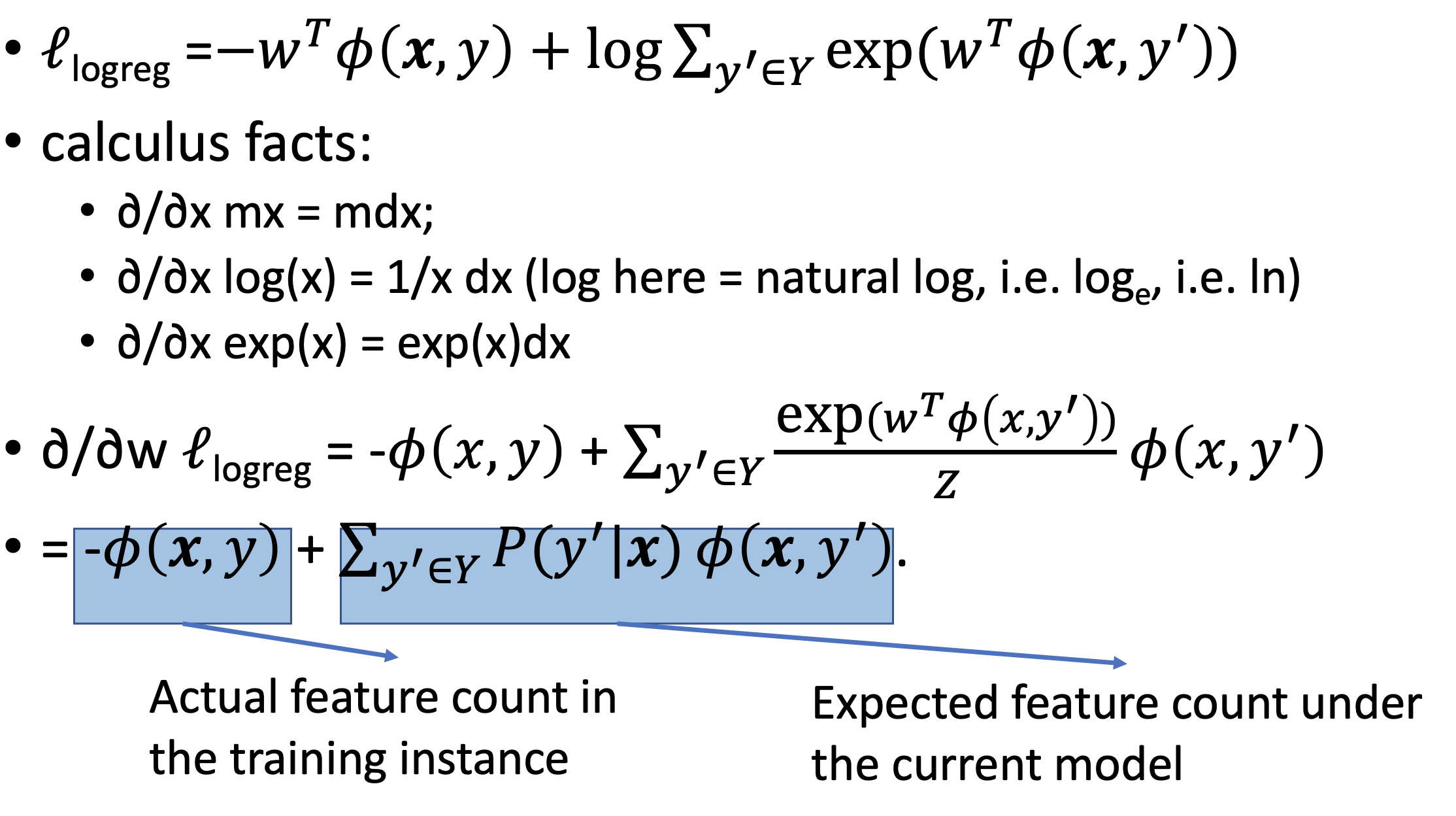
• where z is the sum over the classes ie the 2nd part of the loss
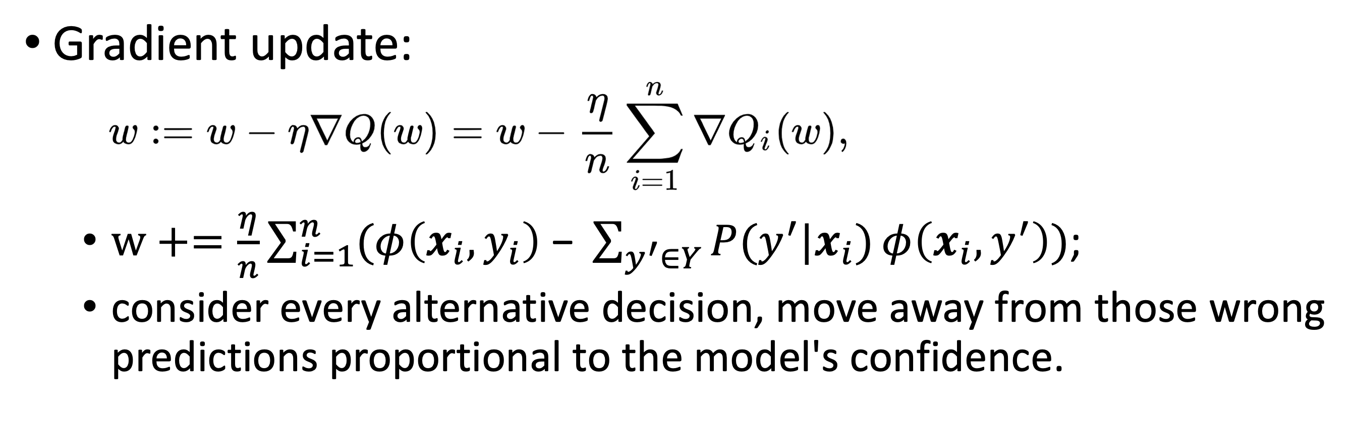
• and the weight update is:

  Differences

•