3 - Linear Algebra for Graphics
ucla | CS 174A | 2024-01-16 18:29
Table of Contents
- Point Arithmetic
- Affine Transformations
- Vector Representations
- Interpolation
- 3-D Rendering
- Matrix Arithmetic
Point Arithmetic
- $P_1-P_2=\vec V$
- $\alpha P_1=P$
- idea: scaling a point makes sense for affine transformations but not for linear combinations
Affine Transformations
\(P=\alpha_1 P_1+\alpha_2 P_2\) where \(\alpha_1+\alpha_2=1\)
Parametric Form of a Line
\(L_2=(1-t)P_1+tP_2\)
- where $L_2$ denotes a 2-D line
- $0\le t\le 1$ -> finite edge
- $\lambda \le t$ -> semi-infinite ray
- $t\in \mathbb R$ -> infinite line
Constraints
- given a convex region defined by some $n$ points $P_i$ and $n$ parameters $\alpha_i$ on the same plane (a planar polygon)
- Affine constraint
- given a point as a parametric sum of points \(P=\sum_i^n\alpha_i P_i\)
- the resulting point will lie on the plane \(\sum_i^n \alpha_i=1\)
- Convex constraint
- homogeneous representation of points and vectors for graphics: add a 4th dimension, 0 = vector, 1+ = point e.g., \(\vec v = (v_1,v_2,v_3,0)\quad P=(p_1,p_2,p_3,1)\)
Affine Transformation of Homogeneous Tuples
- math works the same, but now point arithmetic makes sense \(\alpha X +\beta Y = \big(\alpha X_i+\beta Y_i,...,\alpha+\beta\big)\)
Interpolation
Linear Interpolation of 2 points (parametric line)
\(P_{\text{interp}}=(1-\alpha)P_1 + \alpha P_2\)
- values of $\alpha\in(0,1)$ interpolate a point within the edge made by the 2 points
- values of the parameter outside of this bounds will interpolate points on the line made by these 2 points
- treating the parameter as a unit of time can animate the line as the parameter changes
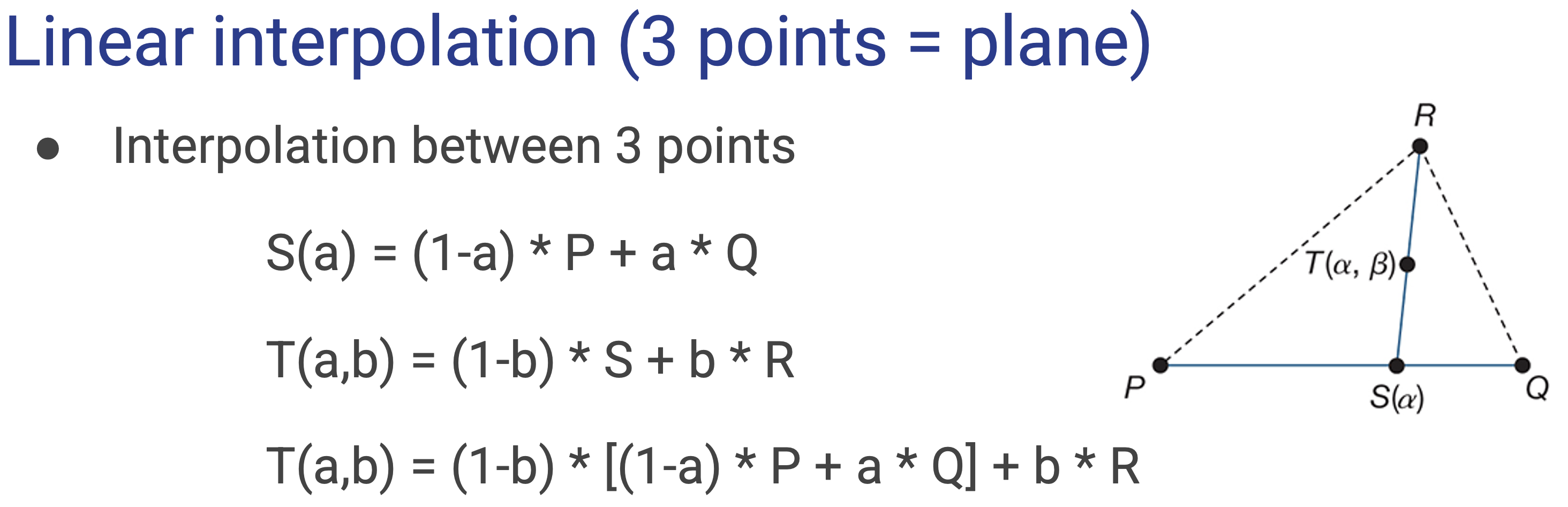
Planar Interpolation of 3 points (parametric polygon)
- given a planar polygon of 3 vertices PRQ triangle, we can interpolate dimensionally
- linear interpolation bw 2 points \(S(\alpha) = (1-\alpha)P + \alpha Q\)
- planar interpolation (point by point) \(T(\beta) = (1-\beta)S+\beta R\) \(T(\alpha,\beta)=(1-\beta)\cdot\bigg((1-\alpha)P+\alpha Q\bigg) + \beta R\)
3-D Rendering
- use triangles to represent shapes bc closed, convex, planar, simple, and optimal in vertices
- interpolate triangles to fill and tesselate shapes to make structures
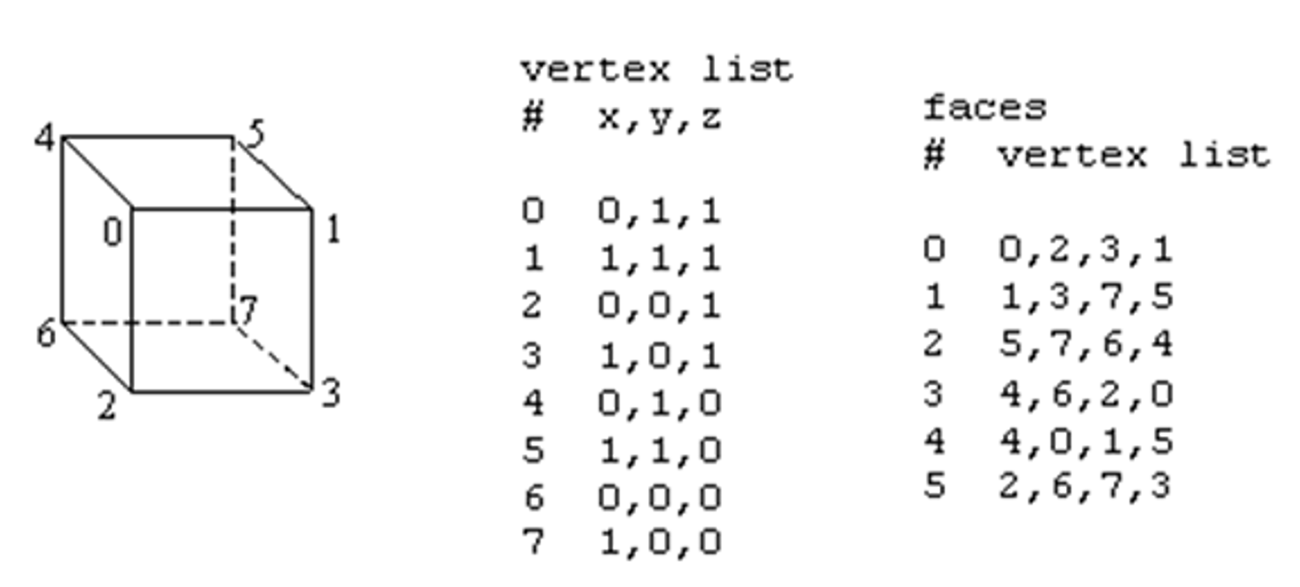
- create 3-d objects using indexed face/data sets
- give an indexed list of vertices coordinates
- then give an indexed list of faces using prev list in counter-clockwise order (to make normals outward pointing)
- these point lists can be loaded into a matrix to parallelize then load onto GPU for fewer communication calls
Matrix Arithmetic
- we make homogenous representations using quaternions
- all except scale and shear are orthonormal matrices i.e., rigid body transformations
- all are affine transformations
- they maintain collinearity
- maintains planarity
- maintain parallelism
- maintain edge-length ratios
- the final transformation matrix made of a series of products of transformations can be seen to be composed only of rigid body transformations IF the smaller 3x3 (top left) of the final matrix is orthonormal
- the inverse of orthonormal matrices is the transpose of the matrix \(A^{-1}=A^T\quad\text{iff.}\quad \text{$A$ is orthogonal}\)
- pure translation is commutative
- pure rotation is commutative and additive
- a linear combination of them is not commutative
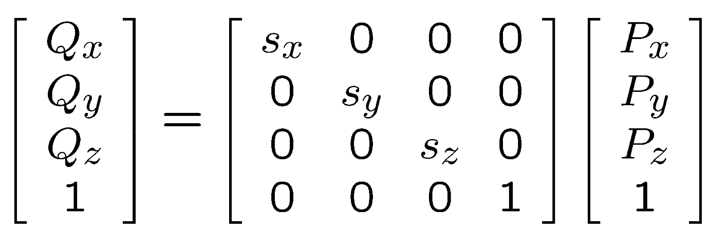
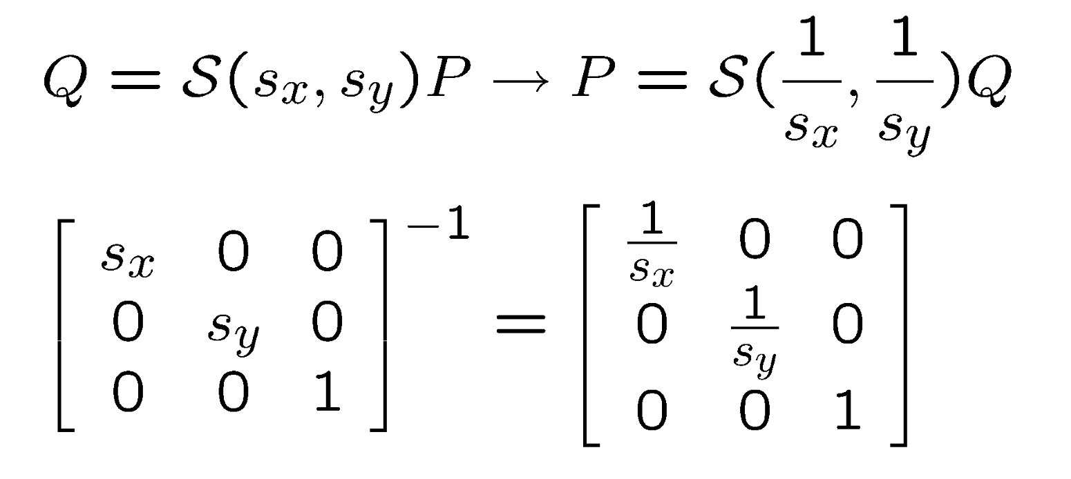
Scaling
- scaling wrt to origin, use diagonal scaling matrix to scale unit vectors \(\begin{pmatrix}x' \\ y'\end{pmatrix}=\begin{pmatrix}S_x & 0 \\ 0 & _y\end{pmatrix}\begin{pmatrix}x \\ y\end{pmatrix}\)
Inverse
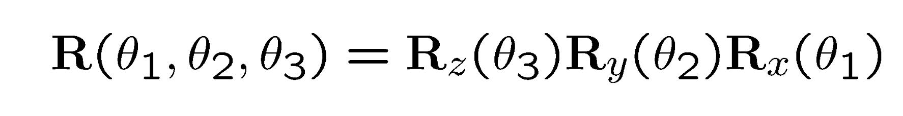
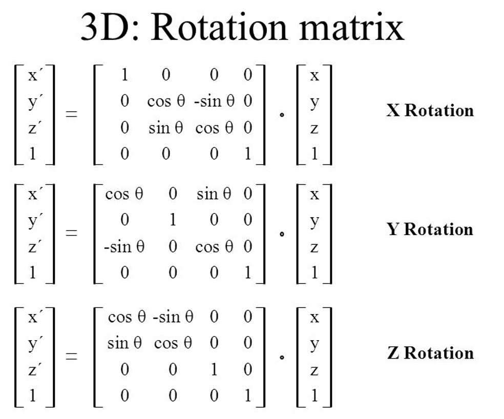
Rotation
- use rotation matrices to rotate a vector by an angle $\theta_x$ off the axis of relevance, e.g. in 2-D about to axis $x$
- 2d representation\(\begin{pmatrix}x' \\ y'\end{pmatrix}= \begin{pmatrix}\cos\theta & -\sin\theta \\ \sin\theta & \cos\theta \end{pmatrix}\begin{pmatrix}x \\ y\end{pmatrix}\)
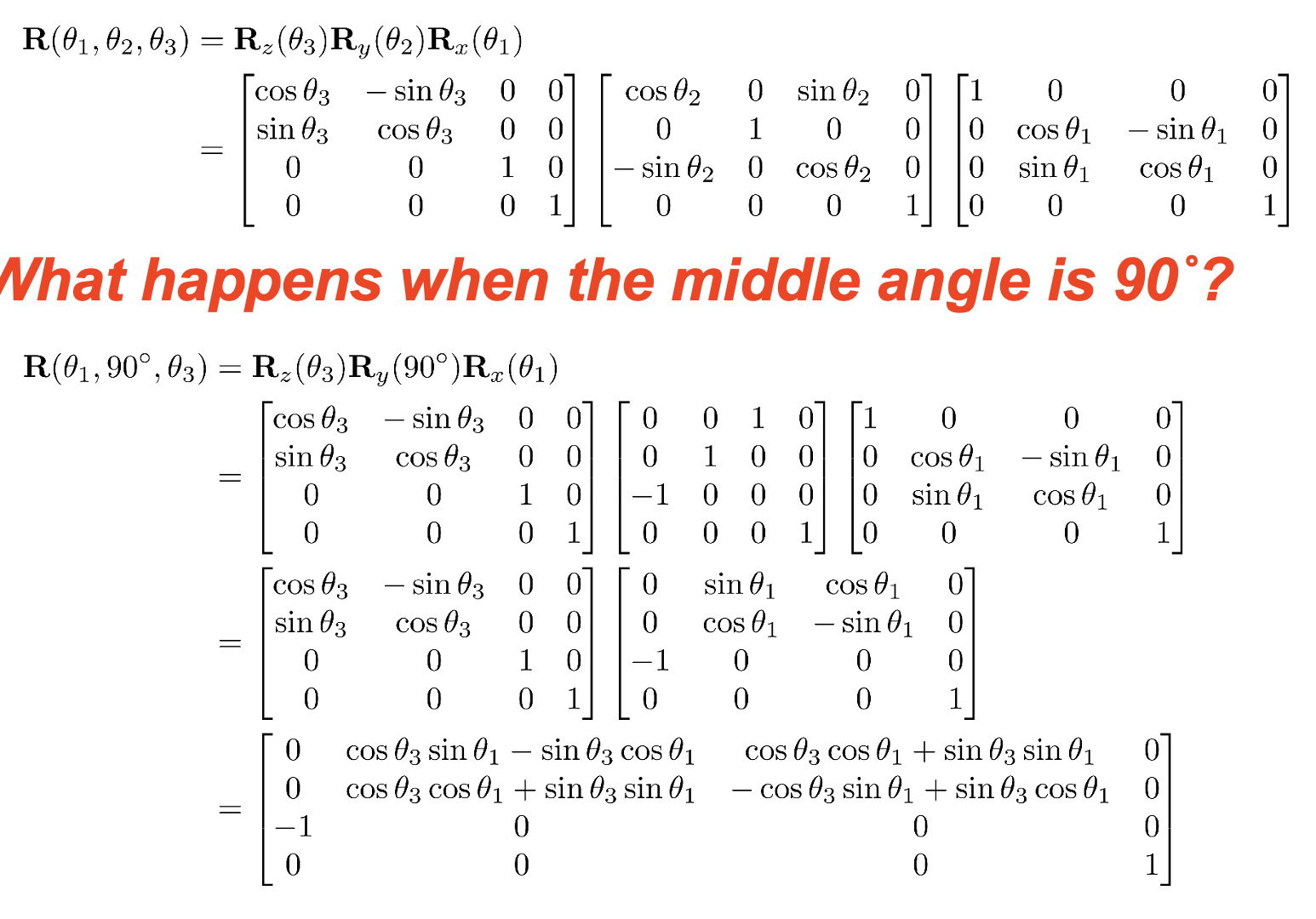
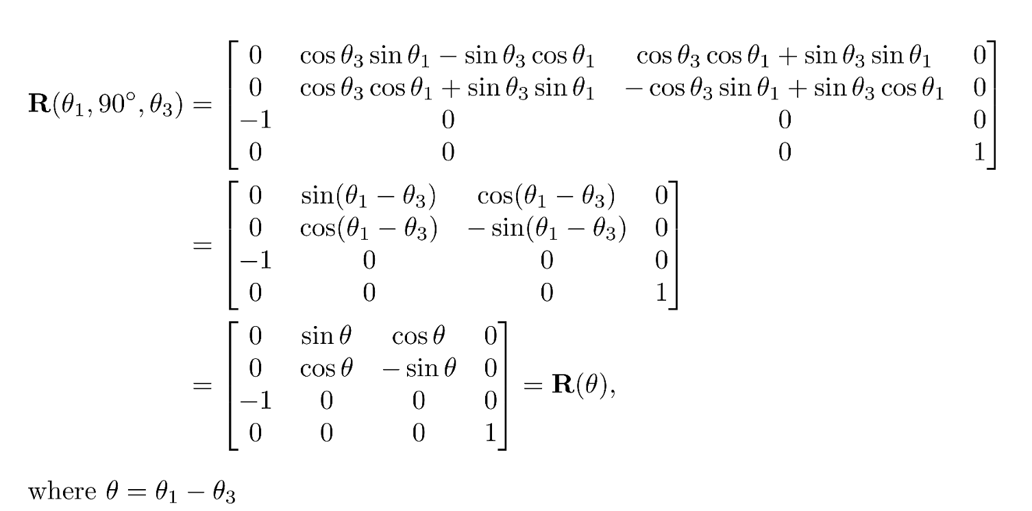
- 3-D representation \(\begin{alignat}{1} R_x(\theta) &= \begin{bmatrix} 1 & 0 & 0 \\ 0 & \cos \theta & -\sin \theta \\[3pt] 0 & \sin \theta & \cos \theta \\[3pt] \end{bmatrix} \\[6pt] R_y(\theta) &= \begin{bmatrix} \cos \theta & 0 & \sin \theta \\[3pt] 0 & 1 & 0 \\[3pt] -\sin \theta & 0 & \cos \theta \\ \end{bmatrix} \\[6pt] R_z(\theta) &= \begin{bmatrix} \cos \theta & -\sin \theta & 0 \\[3pt] \sin \theta & \cos \theta & 0 \\[3pt] 0 & 0 & 1 \\ \end{bmatrix} \end{alignat}\)
- Quaternion representation
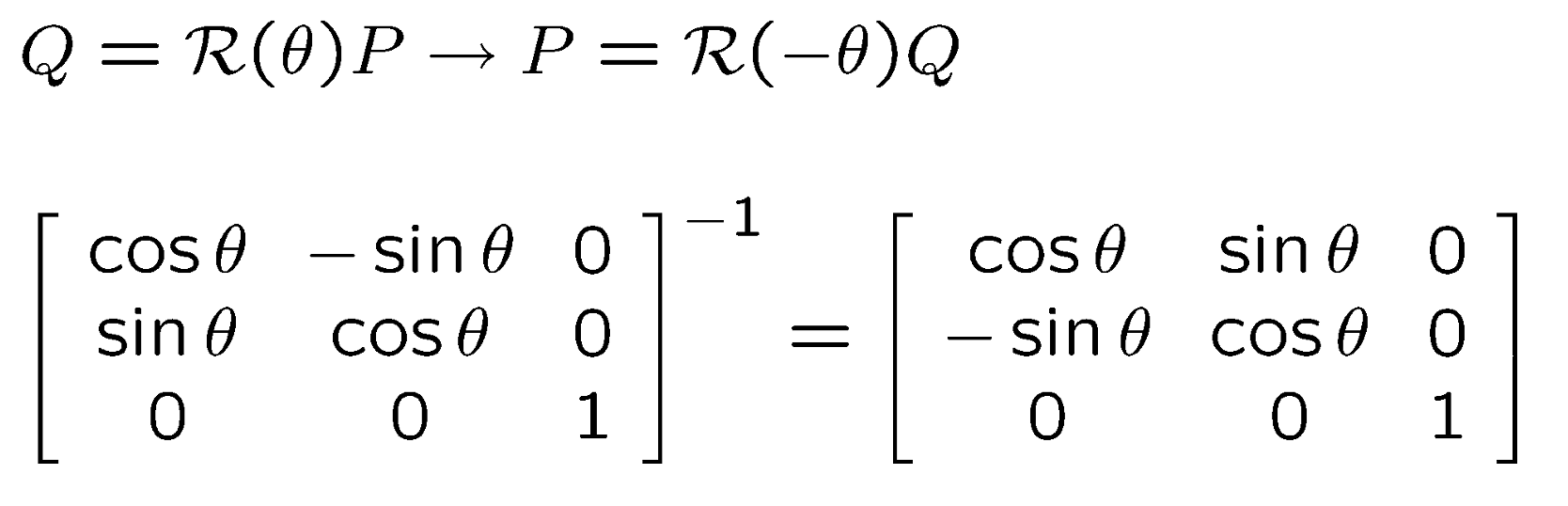
Inverse
- pure rotations are also orthonormal, so simply taking the transpose of the transformed/rotated points will give the inverse
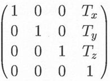
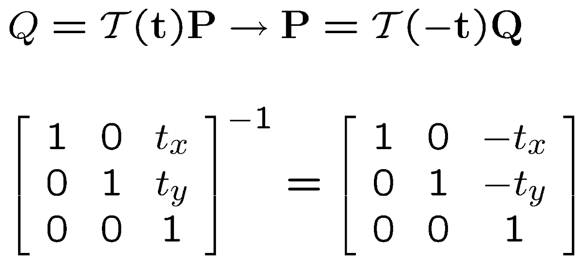
Translation
- use quaternions
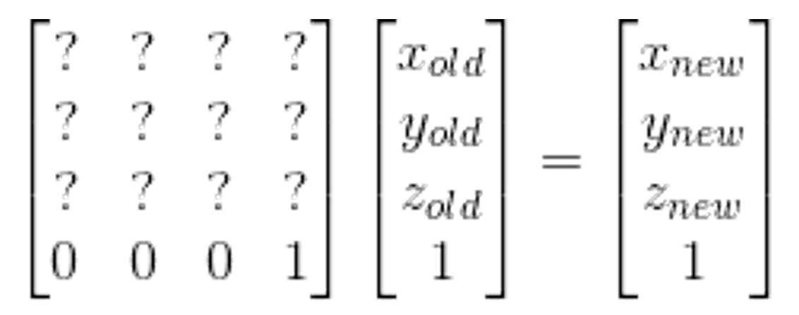
- such that the translation matrix is
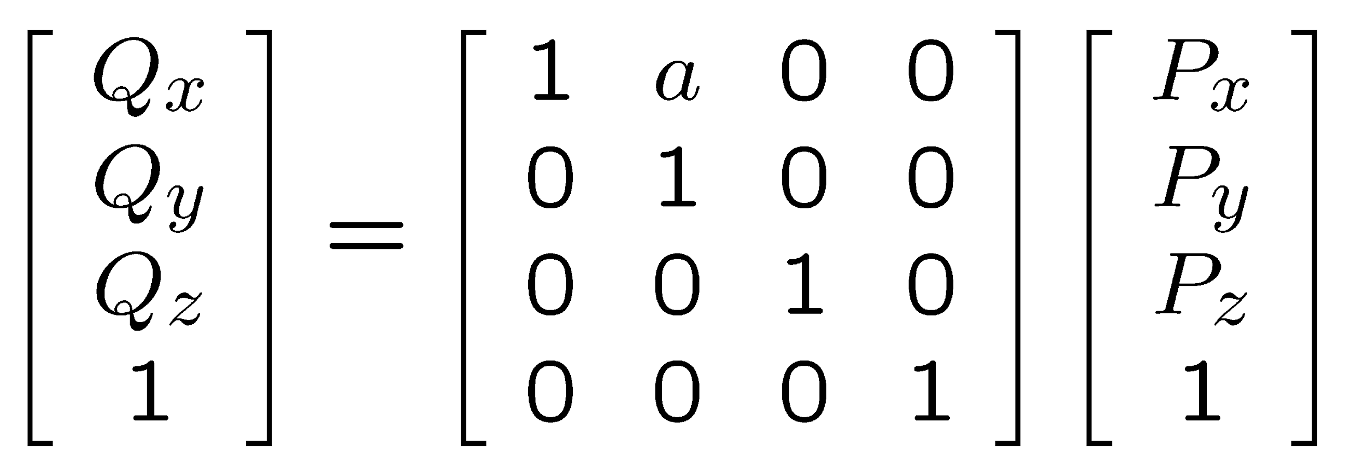
Shear
- along x-axis
- along y-axis \(\begin{pmatrix}x' \\ y' \\ z' \\ 1\end{pmatrix}= \begin{pmatrix}1&0&0&0\\b&1&0&0\\0&0&1&0\\0&0&0&1\end{pmatrix}\begin{pmatrix}x \\ y\\z\\1\end{pmatrix}\)
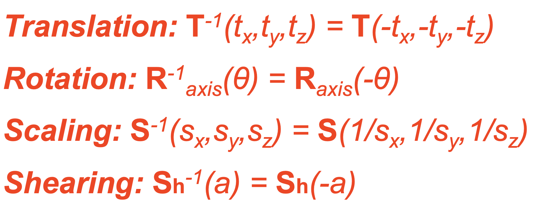
Inverse
- inverse in x-axis
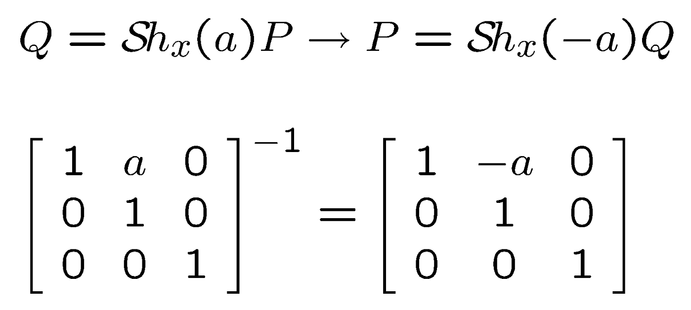
Inverse of Transformations