1 - Adversarial Robustness
ucla | ECE 209AS | 2024-04-01 17:16
Table of Contents
- Adversarial Perturbation (For Red-Teaming)
- Robustness
- Attacks
- Projected Gradient Descent
- Blue-Teaming against Adversarial examples
Adversarial Perturbation (For Red-Teaming)
- Geometric perturbation - rotating, flipping images to misclassify, e.g. MNIST 7 -> 3 by rotating
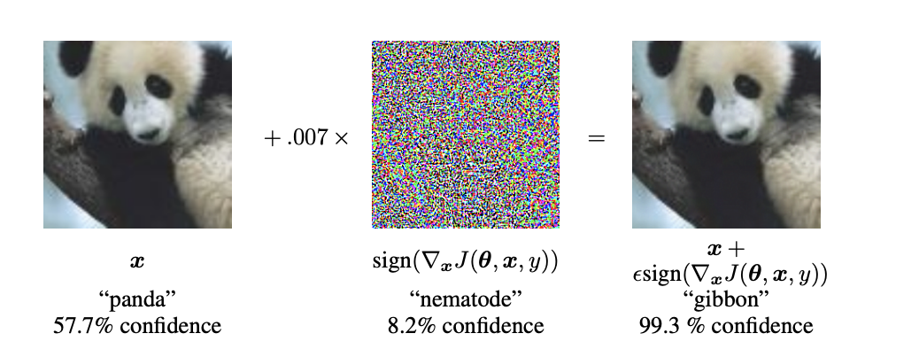
- Noise - overlay noise onto images to misclassify, e.g.
- adding a destructive sentence to language inputs to misgenerate
- concat noise to RLHF to misclassify/mispredict action of the RL model
- can also be used to find better, nonlinear classification metrics
Robustness
- outputting correct outputs for all inputs
- large input pace -> local robustness: outputting correct outputs on inputs similar to inputs in the training set -> accuracy
- Accuracy is not a great metric on the test set, though, due to the prob distribution of samples, so there are some low prob examples that have never been seen and will thus have low classification accuracy.
Attacks
- targeted attacks - misclassify a specific label to some other label or any other label
- untargeted attack - misclassify all labels to any incorrect label
- e.g. we define a NN
- then given a target
- then an adversarial example is given as
- i.e., misclassification
Types of Attacks
- white box attacks - attacker knows about model arch, params, etc.
- black box attacks - attacker knows arch (layers) but not params (weights)
Fast Gradient Sign Method (FGSM)
- From the previous example:
- I.e., we grab the gradient w.r.t. the inputs for the bad (misprediction) class
- Because we want the loss of misclassification to go down (i.e. making it misclassify more), we subtract the loss so we move towards a lower loss -> optimizing misclassification
Perturb the input:
- Then we check and grab losses if
Untargeted FGSM
- For the correct class
- perturb positively because we want the loss to go up i.e. maximize loss and minimize correct predictions
- then check
Concept of distance
- we want small but effective perturbations for attacks so we don’t perturb the image to much and make a significant change
so we need some metric for distance: norms to find sim x-x’ _p<\epsilon$$ we usually look at L inf to find maximum noise and then reduce that: $$ \vec x _\infty=\max( x_1 ,…, x_n )$$ - thus we want noise
The optimization problem
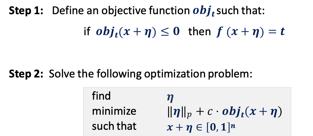
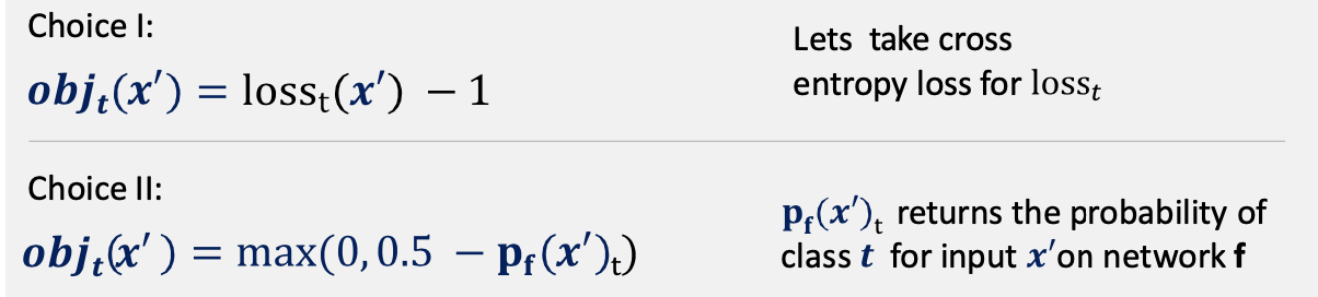
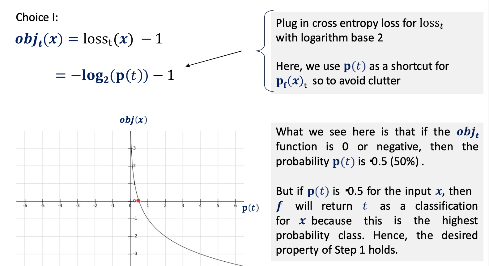
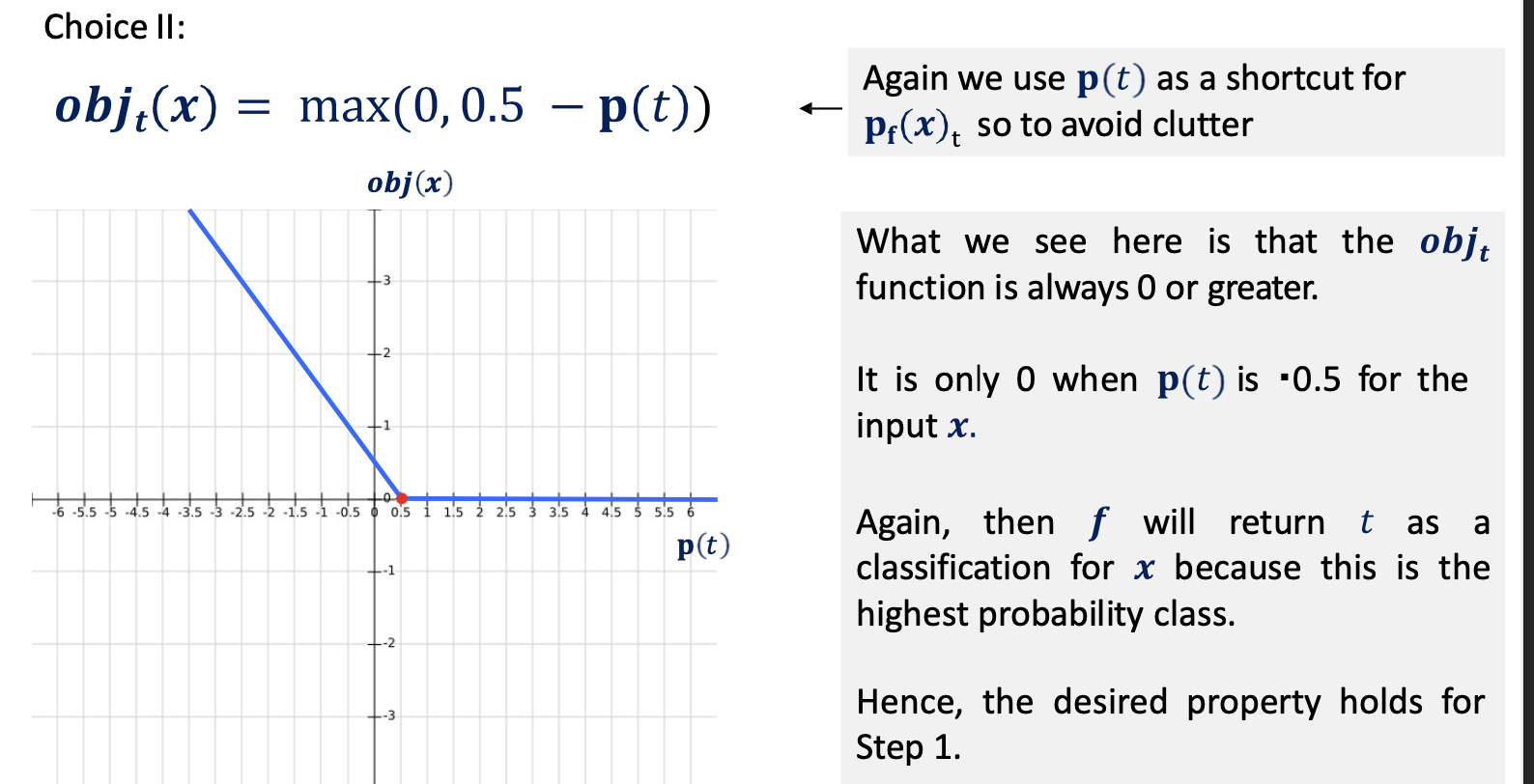
- Now, we consider some functions for obj that satisfy the constrained optimization problem:
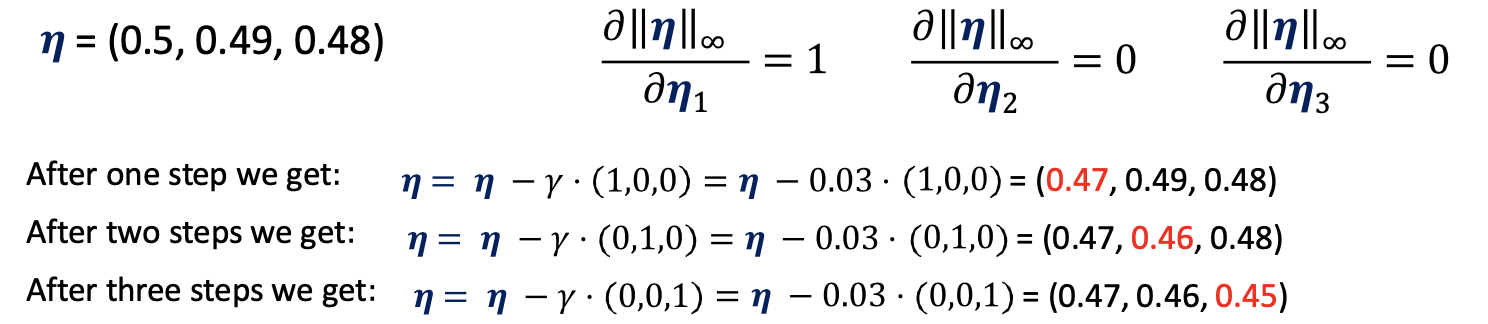
- gradient updates are circular in updating the objective function due to oscillation across the elements of the perturbation
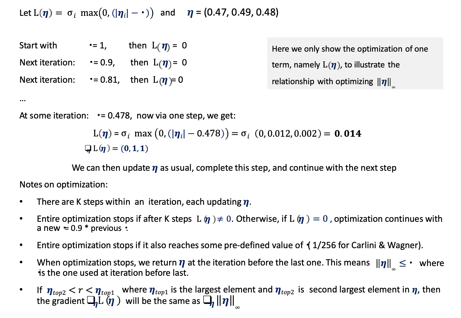
we can solve this issue using regularization of the perturbation by \vec\eta _{\infty}\to\sum_i\max(0, \eta -\tau)$$ - we see when applying
Projected Gradient Descent
- we project all noise values outside some bounding box to make the optimization faster and easier to update [TODO: insert clip function from slides]
Working Example
- [insert slides on PGD w/ example
Implementation Details
- projection is linear op for
- finding efficient project spaces (convex regions) is an open problem - domain-dependent
- early stopping is usually implemented
- we also usually do a random walk from the initial random perturbation (usually ends up inside the clipped box instead of the corner example) instead of taking FGSM off the bat
Tradeoff
[insert table from slides here]
Blue-Teaming against Adversarial examples
- models train on adversarial examples now
- measure both test accuracy and adversarial accuracy on adversarial examples and optimize model -> these accuracies are usually inversely proportional and may train oppositely (adv acc inc <-> test acc dec)
- making robust classifiers
- start with mini-batch B of dataset D
- compute
Solution to empirically robust models
- the loss after adversarial training reduces the loss and frequency space to a very marginal area which limits the number/space of adversarial examples
- [insert slide on loss change after adversarial training]