01 - Final Review

ucla | CS M148 | 2024-12-05

PCA

principal component analysis - an unsupervised, dimensionality reduction method
computes orthogonal linear combinations that maximize variance of data features relative to the origin
can be done via SVD or Eigen decomposition (but this requires a square matrix (i.e. padding))
Standardization
method of mean-centering and Stdev-scaling data
Normalization - centering mean at 0, scaling to -1,1
SVD
singular value decomposition - decomposes dataframe s.t. $X = U D V^{T}$
- if X is $m \times n$ where $m$ is samples and $n$ is features, then
- $U$ is of shape $m \times m$
- $D$ is $m \times n$ - usually the top half ( $n \times n$ ) is diagonally non-zero, the bottom half is usually 0s
- $V$ is $n \times n$
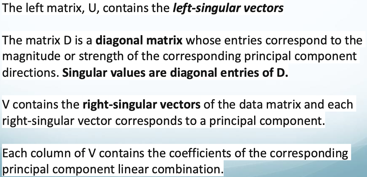
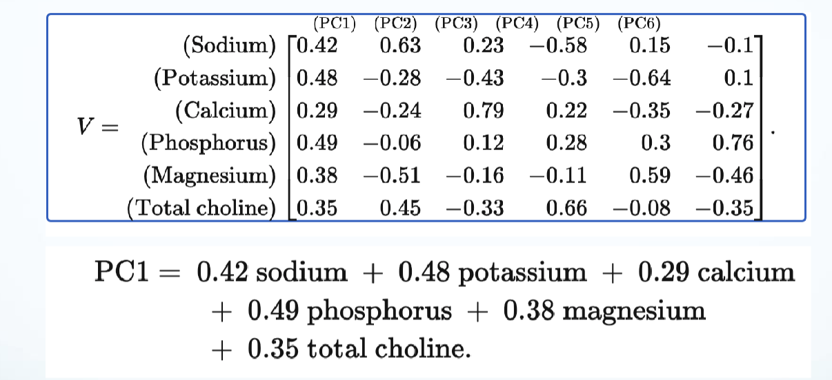
e.g., variable loadings given by right singular vectors:
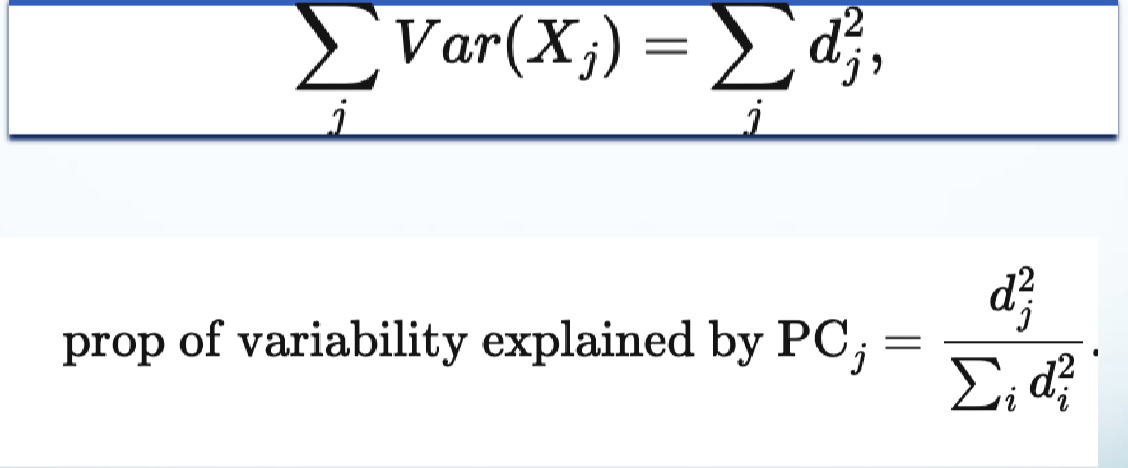
Explained Variance
where $d$ is an element of the singular value matrix ( $D = Σ$ )

Clustering

divisive clustering - put all objects in 1 cluster and iteratively split
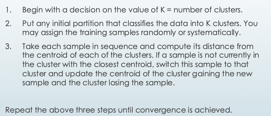
- e.g., k-means
- uses a distance metric only (basically mean linkage with centroids at means of data in the cluster)
agglomerative/hierarchical clustering - begin with singleton clusters and merge until 1 cluster
- can construct dendrogram and cut at some height to result in a number of clusters
- uses a distance metric AND a linkage metric to link clusters together e.g., ward, single (min), complete (max), mean linkage
  K-means Clustering
iterative, unsupervised, always converges to singleton clusters unless early stopped
K is a hyperparameter
algo
Metrics
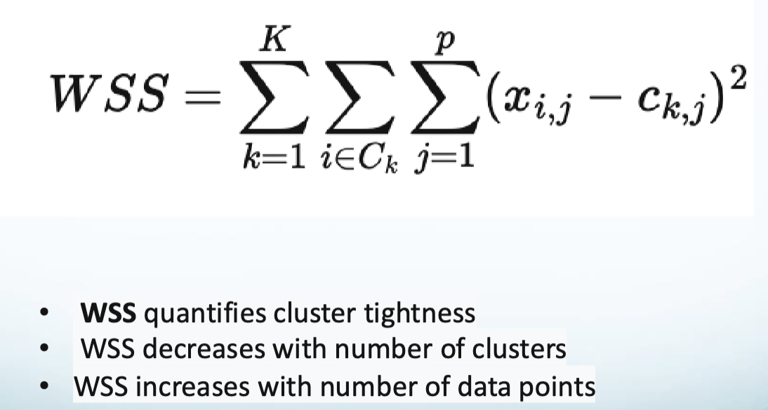
WSS - within cluster sum of squares - metric to measure the quality of a clustering
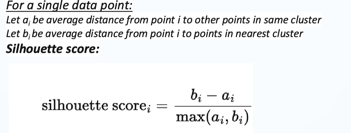
silhouette score - quantifies how tightly each data point is clustered and how distinctly each data point is clustered • Average silhouette scores for each point to get clustering silhouette score
Rand index - metric to compare 2 clustering methods
Adjusted rand - adjusts for expected clustering

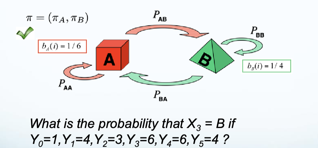
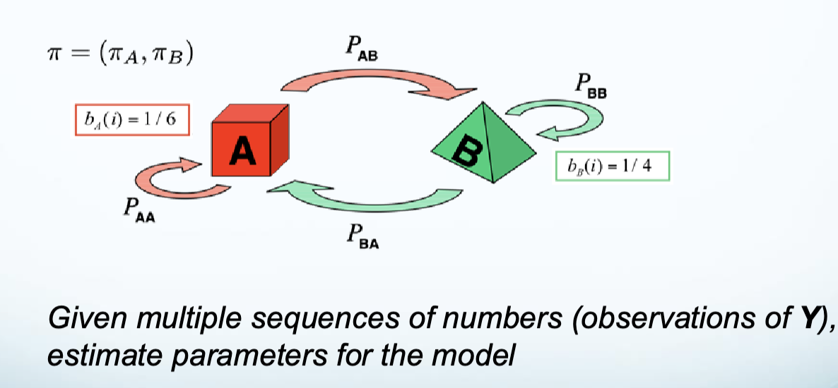
HMM

hidden markov model - a statistical model used to represent systems that are assumed to be a Markov process with unobservable (hidden) states. HMMs are widely used in various fields, including speech recognition, natural language processing, bioinformatics, and more. Here’s a breakdown of the key components and concepts:
allows to deal with time-series data with markov chains
hidden random variables - state of the model
observed variables - outputs of the model

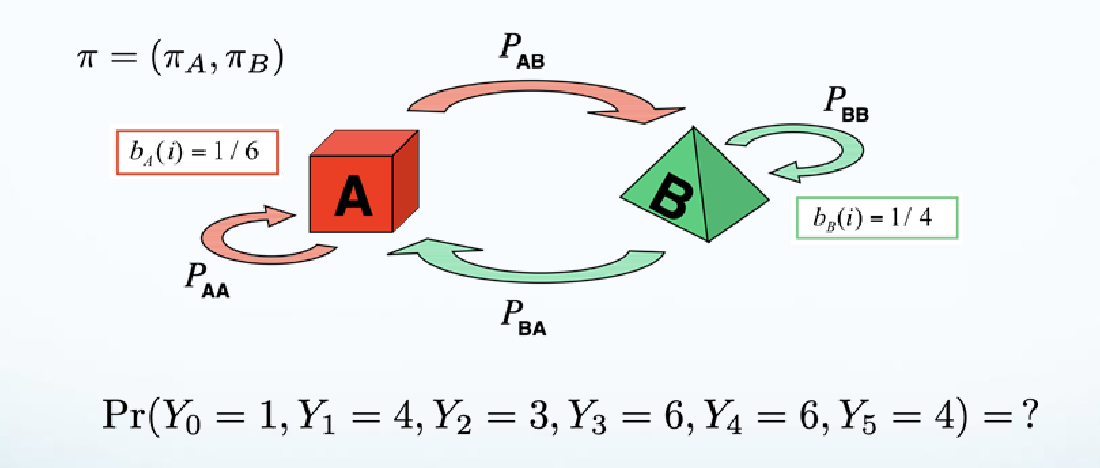
Forward Algorithm Problems

https://youtu.be/9-sPm4CfcD0?si=v_b3Lqy16GfYegXE

e.g. finding the probability of a markov chain from an HMM

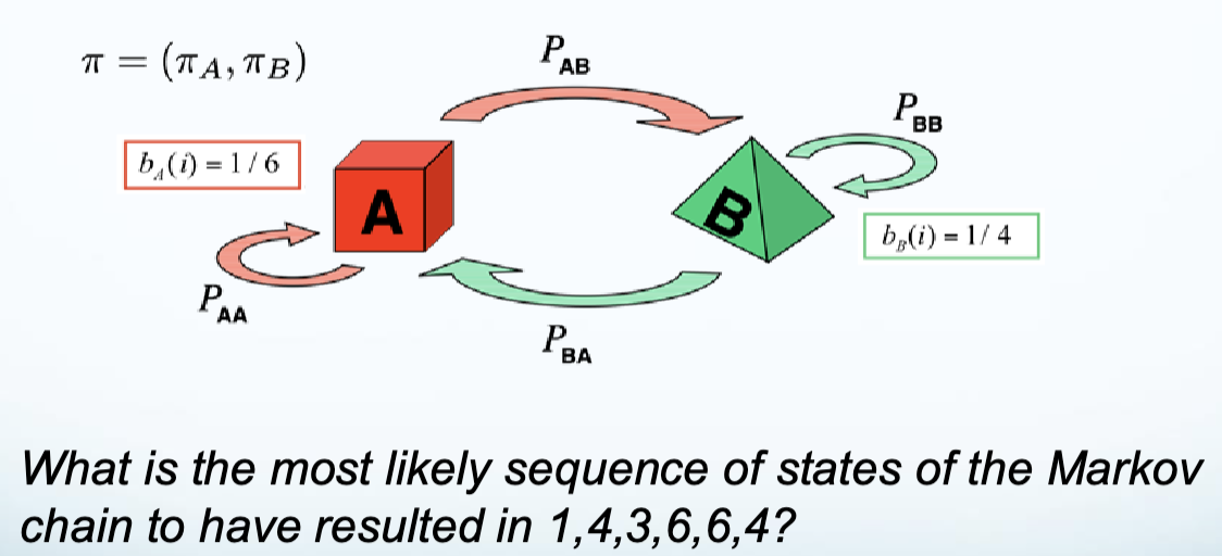
Backward Algorithm (Viterbi) Problems

https://youtu.be/IqXdjdOgXPM?si=95UeWqSNLU4noeC1

e.g., finding the hidden states that result in an output/observed sequence

Forward-Backward Problems

e.g., find conditioned probability given hidden state markov chain

[Optional]Expectation-Maximization (Baum-Welch) Problems

e.g.,

HMM Components

States:
- The model consists of a set of hidden states. These states are not directly observable but can influence observable events.
Observations:
- Each hidden state can produce observable outputs (or emissions). The relationship between the hidden states and the observations is defined by a probability distribution.
Transition Probabilities:
- There are probabilities associated with transitioning from one hidden state to another. This is often represented in a transition matrix, where each entry indicates the probability of moving from one state to another.
Emission Probabilities:
- For each hidden state, there is a probability distribution that defines the likelihood of producing each possible observation.
Initial State Probabilities:
- This defines the probabilities of starting in each of the hidden states.

Markov Property:
- The future state depends only on the current state and not on the sequence of events that preceded it. This is known as the Markov property.
Hidden States:
- The states are “hidden” because they cannot be observed directly. Instead, we infer them based on the observable outputs.

NN

neural network - built on the unviersal approximation theorem - by way of linear combinations with non-linear activations => able to model any deterministic function
MLP - feed forward model, dense, fully connected

Backprop

computes gradients of loss wrt to each parameter (that requires grad)
done via chain rule partial derivatives
can also be done via jacobian

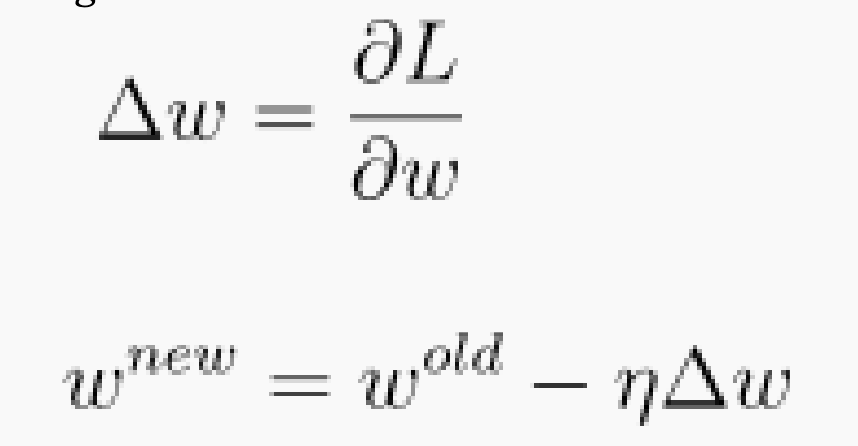
Gradient descent

in this class we subtract the earning rate $η$ times the gradient
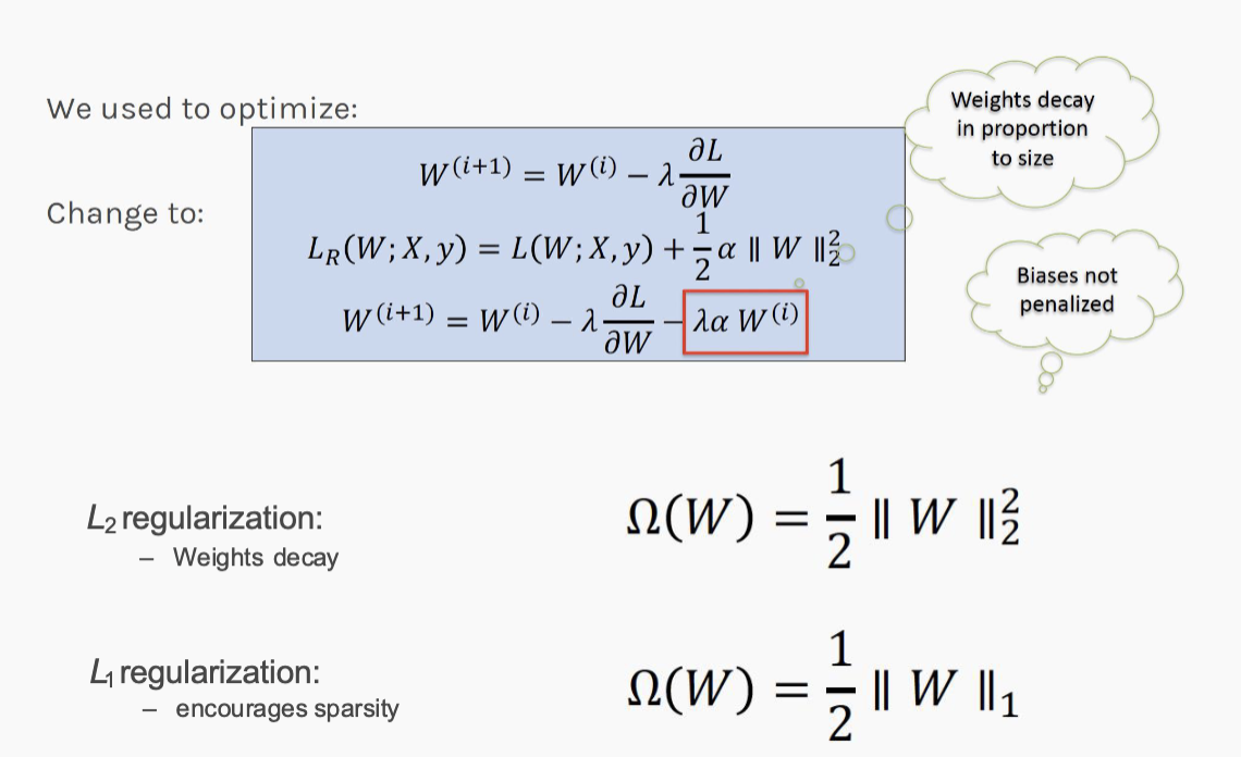
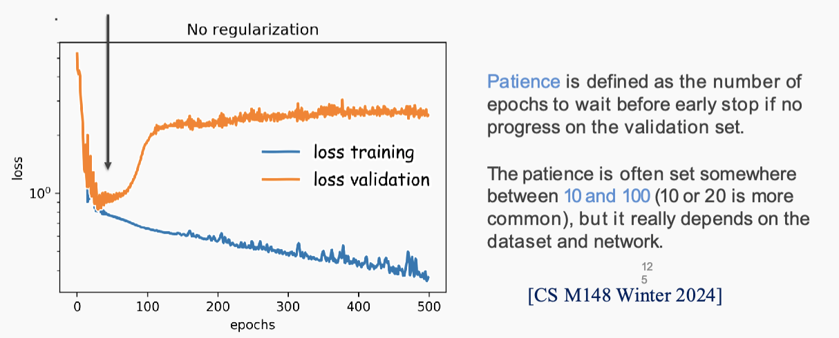
Regularization
methods: norm penalties (standard), early stopping, data augmentation, dropout and the like
Norm penalties
early stopping, stop and train and val loss divergence
data augmentation - adding “fake” data to data set e.g., via image transformations/filters, dataset bootstrapping (random selection w/ replacement), gaussian mixture models (used as generative model)

Random Forests

ensemble method that ensembles many decision trees
trains each tree with a different random bootstrap sample
sometimes each random forest given a different subset of features

Bagging

bootstrap aggregation - train several models on bootstrapped datasets and average results

Dropout

randomly set some neurons and connected weights to zero during training at some time to prevent overfitting that single node/weight
usually dropout some fraction of neurons
also an ensemble method beause dropping out treats each neuron as its own classifier

Model Trust

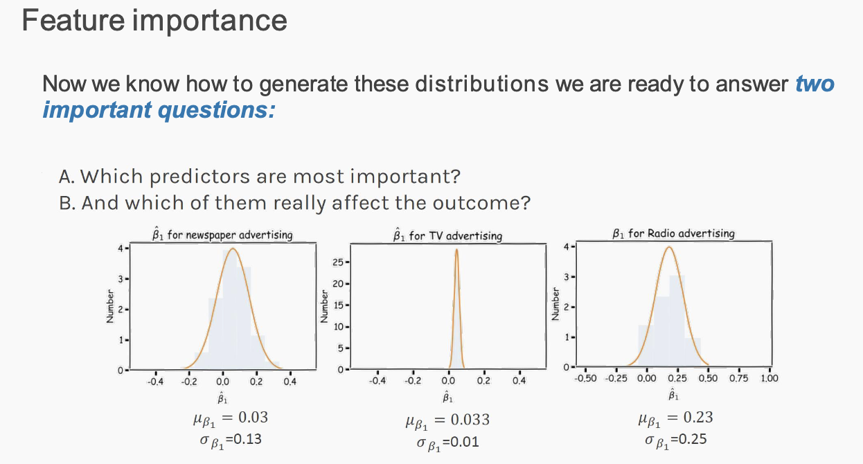
Note: hypo testing for NNs is infeasible bc requires retraining the model when adjusting the features even slightly

Shapley Values

Shapley values are a concept from cooperative game theory that provide a way to fairly distribute the total gains (or costs) among players based on their individual contributions to the overall outcome. Named after Lloyd Shapley, who introduced the concept in 1953, Shapley values have applications in economics, political science, and machine learning, particularly in the context of feature importance in predictive models.

Key Concepts

Cooperative Game:
- In a cooperative game, players can form coalitions and work together to achieve a better outcome than they could individually. The total value generated by the coalition is typically shared among the players.
Value Function:
- The value function assigns a value to each possible coalition of players, representing the total payoff that the coalition can achieve.
Marginal Contribution:
- The marginal contribution of a player is the additional value that the player brings to a coalition. For example, if a coalition of players can achieve a value of ( V(S) ) and adding player ( i ) to this coalition increases the value to ( V(S \cup {i}) ), then the marginal contribution of player ( i ) is ( V(S \cup {i}) - V(S) ).

Shapley Value Calculation

The Shapley value for a player $(i)$ is calculated by considering all possible coalitions that can be formed without player $(i)$ and determining how much player $(i)$ contributes to each coalition. The formula for the Shapley value $ϕ_{i}$ of player $i$ is given by:

ϕ_{i} = \sum_{S \subseteq N ∖ {i}} \frac{| S |! \cdot (| N | - | S | - 1)!}{| N |!} \cdot (V (S \cup {i}) - V (S))

Where:

( N ) is the set of all players.
( S ) is a subset of players not including player ( i ).
( S ) is the number of players in coalition ( S ).
( V(S) ) is the value of coalition ( S ).
The fraction represents the weight of the contribution based on the order in which players join the coalition.

Properties of Shapley Values

Efficiency:
- The total Shapley values of all players sum up to the total value generated by the grand coalition (all players together).
Symmetry:
- If two players contribute equally to every possible coalition, they receive the same Shapley value.
Dummy Player:
- If a player does not contribute anything to any coalition (a “dummy” player), their Shapley value is zero.
Additivity:
- If two games are combined, the Shapley value of a player in the combined game is the sum of their Shapley values in the individual games.